Understanding Softmax Temperature

The Softmax function re-normalizes values so they become a probability distribution (sum to 1). In order to achieve this, the softmax function takes three steps. Let’s take a look at this function from multiple perspectives. If you want to follow or play around, the plots for this post were generated using this notebook.

Here’s the formula: \(\mathcal{S}(x_i)=\frac{e^{x_i}}{\sum_{j=1}^{i}{e^{x_j}}}\)

Here’s the python code:

def softmax(x):
    e_x = np.exp(x - np.max(x))
    return e_x / e_x.sum()

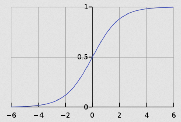
And here it is, plotted for visual inspection:

So, let’s break it down with an example. I’m going to start with a random distribution x and play around with it. Next, I show the three consecutive steps of the softmax: substracting the max, exponential, and normalizing (complete softmax function).

x = get_random_array()
plot_multiple_bar_plots([x,x - np.max(x),np.exp(x - np.max(x)),softmax(x)],
                        [0,-1,0,0],
                        [1,0,1,1],
                        ["Original Distribution","x - np.max(x)","np.exp(x - np.max(x))","softmax(x)"])

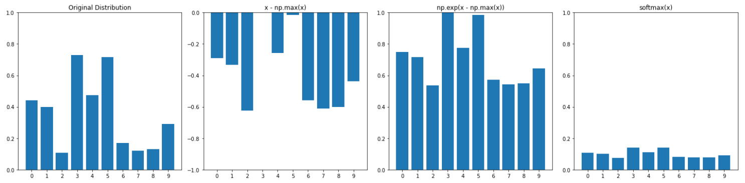
Note that the second graph has the vertical axis on negative values. There are a couple of things to highlight here. The first step transforms all values into negative values by substracting the maximum, all except the maximum, which turns to 0 (spoiler alert, this will make it the maximum value when taking the exponential, as it will get mapped to 1). Then, the second step (\(e^x\)) is in charge of mapping back the values into a range between 0 and 1. This is due to the shape of the exponential funcion:

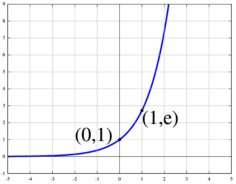
As you can see, all negative values are mapped to positive values that are smaller than or equal to 1.

Now, whith that in mind, let’s introduce temperature (\(\mathcal{T}\)). Temperature is generally applied by dividing \(x\) in the softmax formula, resulting in \(\mathcal{S}(x_i)=\frac{e^{x_i/\mathcal{T}}}{\sum_{j=1}^{i}{e^{x_j/\mathcal{T}}}}\). In this sense, we observe three scenarios. 1) Using temperature equal to 1 leaves the distribution unchanged; 2) Using a temperature greater than 1, which will be equivalent to dividing the values of the distribution; and 3) Using a temperature positive and smaller than 1, which is equivalent to multiplying the values of the distribution. Let’s take a look at different values and how the distribution changes:

1. Large temperature.

   plot_multiple_bar_plots([x/1,x/2,x/5,x/50],0,1,
                        ["$\mathcal{T}=1$","$\mathcal{T}=2$","$\mathcal{T}=5$","$\mathcal{T}=50$"])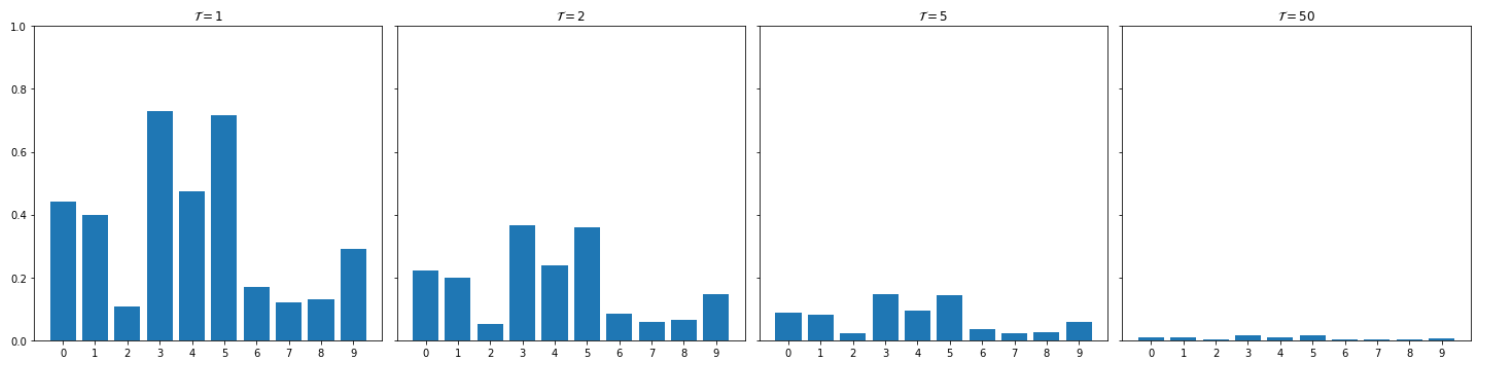
   

   

2. Small temperature.

   maxy=10
   plot_multiple_bar_plots([x/0.75,x/0.5,x/.2,x/.1],0,maxy,
                        ["$\mathcal{T}=.75$","$\mathcal{T}=.5$","$\mathcal{T}=.2$","$\mathcal{T}=.1$"])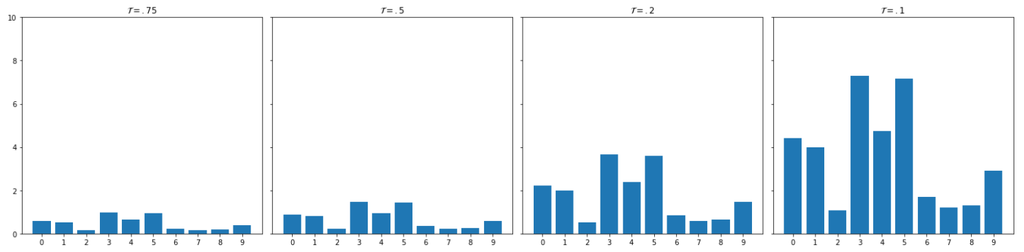
   

   

Note that for this last plot, vertical axis is 10 times larger than for the previous ones. Simply put, it’s a matter of magnitude, a big temperature reduces the magnitude of the values, whereas a small temperature increases it. This opposite behaviour is simply due to the temperature being applied by dividing \(x\).

Ok, so, what effect will this have in the final softmax values? The key to understanding this is the exponential function in the softmax. As it will map values below -2.71828 (approx) very close to 0, the more negative values become, the more values are mapped to almost the same value after the exponential operation. On the one hand, this ends up greatly highlighting the values that were very large to begin with, and are mapped to 0 or close to 0 when the max value is substracted before the exponential. And on the other hand, it will drive to 0 most values that are small in the original distribution, as they become very large in absolute value when the max value is substracted. This is easier to see if we display the multiple steps of the softmax with different temperature values.

1. A large temperature makes most values close to 0 before subtracting the maximum. These are then still close to 0 when negative, resulting in an exponential function that respects those values, i.e. they are still relevant after the exponential. As temperature increases, the output of the softmax will resemble a uniform distribution.

   mult = 1
   temp = 2
   x2 = x / temp
   plot_multiple_bar_plots([x2,x2 - np.max(x2),np.exp(x2 - np.max(x2)),softmax(x2)],
                        [0,-1*mult,0,0],
                        [1*mult,0,1,1],
                        ["Original Distribution","x - np.max(x)","np.exp(x - np.max(x))","softmax(x)"])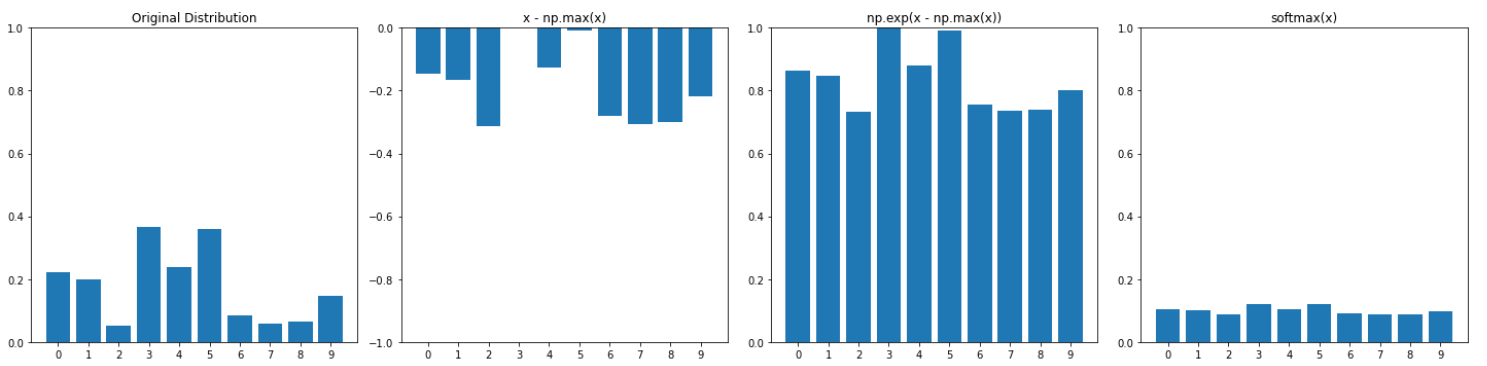
   

   

2. A small temperature, however, causes values to become great, so when the maximum is removed they end up deep into negative space. This results in most values being mapped to 0 by the exponential, so after normalization the only values that still play a role are those close to the maximum of the original distribution. In this sense, a softmax with small temperature highlights only the greater values of the distribution.

   mult = 40
   temp = 0.02
   x2 = x / temp
   plot_multiple_bar_plots([x2,x2 - np.max(x2),np.exp(x2 - np.max(x2)),softmax(x2)],
                        [0,-1*mult,0,0],
                        [1*mult,0,1,1],
                        ["Original Distribution","x - np.max(x)","np.exp(x - np.max(x))","softmax(x)"])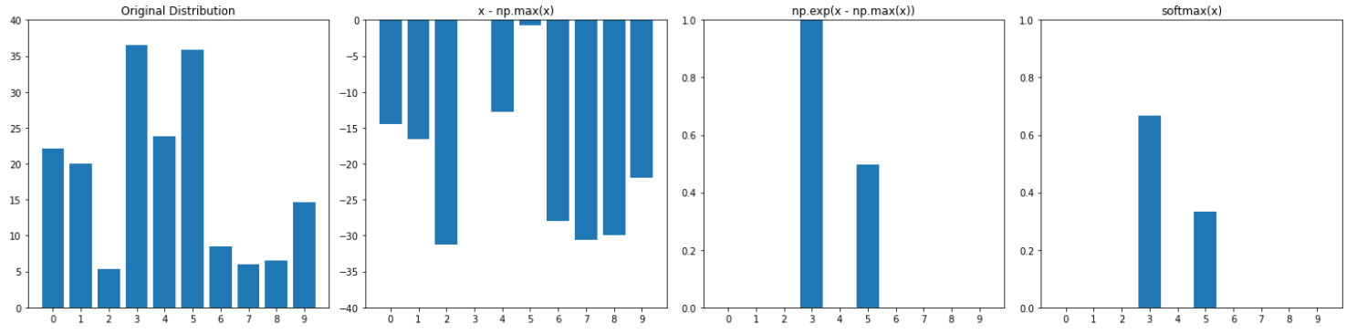
   

   

Note that the first two plots in the last figure have a larger vertical axis. In the end, it all boils down to how the exponential function treats large negatvie values.

This behaviour of the temperature in the softmax helps explain how this value can influence the “creativity” of a chatbot such as ChatGPT. The lower the temperature, the less options it has to choose from when producing the next token, hence become more deterministic and focused, whereas with a higher temperature it becomes more “diverse” and creative, because it weights more options as having a similar weight.